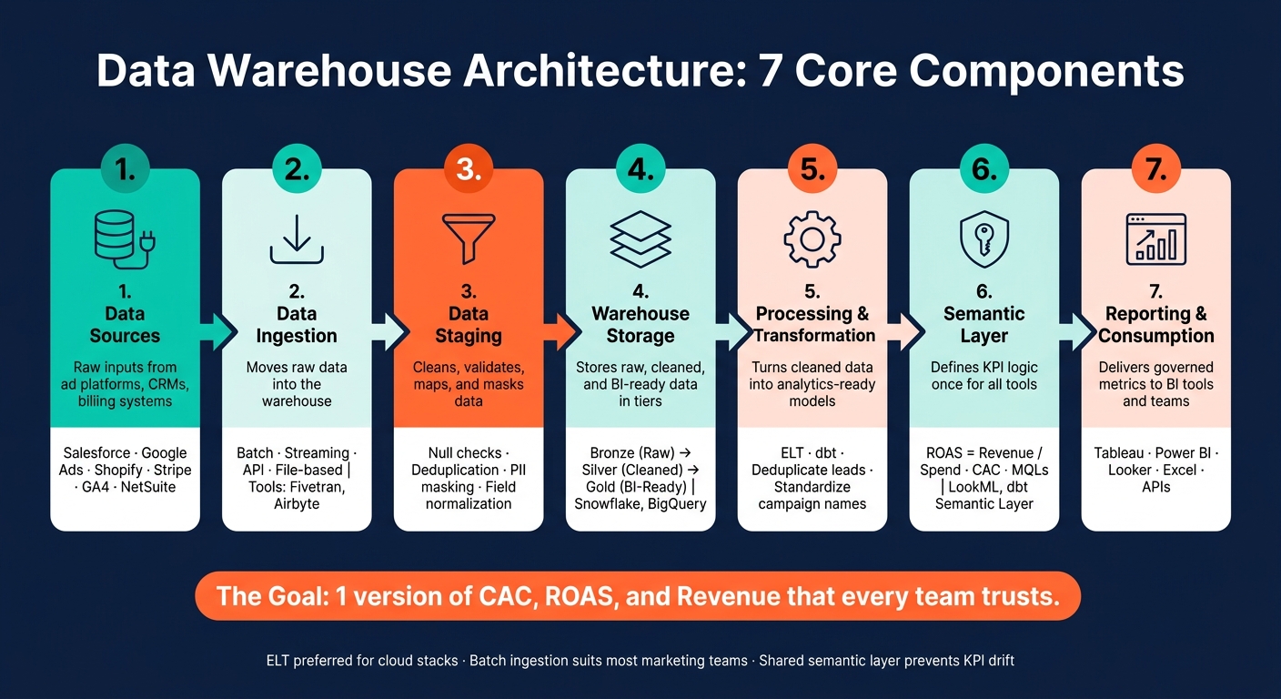
If your team gets different CAC, ROAS, or revenue numbers, the issue is usually the stack - not the math. I’d reduce this topic to 7 parts: sources, ingestion, staging, storage, transformation, semantic layer, and reporting.
Here’s the short version:
- Sources pull data from tools like Salesforce, Google Ads, GA4, Shopify, Stripe, and NetSuite.
- Ingestion moves that data into the warehouse through batch, streaming, APIs, or files.
- Staging checks, cleans, maps, and masks data before it reaches reporting models.
- Storage keeps raw, cleaned, and BI-ready data in separate layers.
- Transformation turns source data into usable tables for spend, pipeline, and revenue analysis.
- The semantic layer sets shared KPI logic so CAC, ROAS, and revenue mean the same thing everywhere.
- Reporting puts those governed metrics into top analytics tools for business, spreadsheets, and apps.
A few points matter most:
- Batch loads are enough for most marketing teams. Daily or hourly updates usually cover reporting needs.
- ELT fits most cloud setups because raw data stays in the warehouse for rework and backfills.
- Shared metric logic cuts KPI drift across marketing, RevOps, and finance.
- Idempotent pipelines, schema checks, and row-level access controls help stop bad data and access issues before they hit dashboards.
If I were explaining the article in 1 line, it would be this: good warehouse architecture gives you 1 version of spend, pipeline, and revenue that teams can use without arguing over the numbers.
Data Warehouse Architecture: 7 Core Components Explained
How Data Warehouse Architecture Supports a Marketing Analytics Stack
From source systems to dashboards
Data usually starts in ad platforms, CRMs, and billing systems. It then moves through warehouse layers before anyone sees it in a dashboard. Ingestion pipelines pull that data into a staging area, where it lands raw and unchanged. After that, transformation steps clean it up and shape it into analytics tables. A semantic layer defines metrics once, and reporting tools connect to that layer to show the results.
Each handoff keeps lineage intact and helps keep reporting trustworthy.
Common systems in a U.S. marketing stack
These layers usually begin with a familiar set of U.S. marketing systems.
| Source Type | Common Platforms | Data Added |
|---|---|---|
| CRM | Salesforce, HubSpot | Lead, opportunity, and account activity data |
| Ad Platforms | Google Ads, Meta Ads, LinkedIn, TikTok | Spend, impressions, clicks, and conversions |
| Website analytics tools | GA4, Adobe Analytics | Page views, session data, and conversion events |
| E-commerce/Billing | Shopify, Magento, Stripe | Orders, refunds, and product-level revenue |
| Finance / ERP | NetSuite, QuickBooks | Costs, margins, and P&L data for ROI reporting |
Each platform has its own schema and refresh cadence. Google Ads may report daily campaign totals, while Stripe records individual transaction timestamps. The warehouse lines up those cadences and schemas so the reports stay comparable.
Why architecture matters for CAC, ROAS, and revenue reporting
CAC and ROAS only work when ad spend connects cleanly to CRM and revenue data. Without a warehouse, teams often calculate them from different systems and end up with mismatched numbers.
Good architecture also deals with the messiness of live data. Campaign names can change in the middle of a quarter. Slowly Changing Dimensions (SCD Type 2) keep past labels and stages in place when campaigns or pipeline states shift.
That gives teams reporting they can use for monthly closes, quarterly reviews, and annual planning.
Next, the seven components break that path into distinct layers.
sbb-itb-5174ba0
Main Data Warehouse Components Explained (2025)
1. Data Sources Layer
The data sources layer is the starting point. It pulls in raw data from top analytics tools across ad platforms, CRMs, e-commerce systems, web analytics, finance tools, and support platforms. At this stage, the data stays as-is. No cleanup, no mapping, no modeling. Everything that comes later depends on this layer being complete and untouched.
These systems set the raw inputs the warehouse needs to standardize.
| Source Category | Representative Systems | Data Contributed |
|---|---|---|
| Advertising | Google Ads, Meta Ads | Spend, impressions, clicks, campaign IDs |
| CRM | Salesforce, HubSpot | Leads, deal stages, contact profiles |
| E-commerce/Billing | Shopify, Stripe | Orders, revenue, refunds |
| Behavioral | GA4, Segment | Page views, session data, events |
| Finance | NetSuite | Operating costs, margins, P&L data |
| Support | Zendesk | Ticket volume, resolution time, CSAT scores |
Downstream, those inputs turn into spend, pipeline, and revenue data.
The hard part is that every source speaks its own language. One tool might label a field Cust_ID, while another uses CustomerID. Same idea, different format. That mismatch is exactly why this layer matters.
This layer should create an immutable raw copy, often stored as JSON, Parquet, or CSV files partitioned by ingestion time [1][5]. That gives teams a clean fallback. If a later transformation fails, they can reprocess from the original source data instead of guessing what changed.
The main risks are schema drift and siloed metrics. Schema drift can break ingestion pipelines when a source system changes without notice. Siloed metrics create competing versions of the same number, like "Revenue", across Finance and Marketing.
Use versioned schemas and source contracts to catch breakage before data reaches ingestion [1].
Next, ingestion moves this raw data into the warehouse.
2. Data Ingestion Layer
The ingestion layer pulls data from source systems into the warehouse. After it lands, staging gets it ready for cleanup and validation.
The right ingestion method depends on the job:
- Batch ingestion runs on a schedule. It fits CRM exports, ERP data, and past ad spend from platforms like Google Ads or social media analytics tools like Meta Ads.
- Streaming ingestion moves data nonstop for near-real-time dashboards and live monitoring.
- API-based ingestion uses managed connectors or custom API jobs to pull from ad platforms, CRM, web analytics, email, and ecommerce tools.
- File-based loading brings in CSV, JSON, or Parquet files from cloud object storage.
This layer should land a raw copy of the data, along with load timestamps and lineage. That gives teams a clear record of where the data came from and when it showed up. It also gives later transformation steps a stable starting point.
Two risks do most of the damage here. Duplicate records show up when a failed pipeline job reruns without idempotency. That can inflate metrics like ROAS or CAC. Schema drift happens when a source system renames a field or adds a column. Then downstream transformation pipelines break, and revenue or spend reporting can go sideways.
Use idempotent jobs, schema-change alerts, and pipeline monitoring. From there, the raw load moves into staging for validation and cleanup.
3. Data Staging Layer
The staging layer is where raw data gets cleaned, checked, and lined up before it lands in warehouse tables.
Think of it as a checkpoint between ingestion and storage. This is where business rules get applied so the data is clean, consistent, and complete. Null values are flagged, duplicates are caught, date formats are normalized, and field names from different systems are mapped into one shared structure. For example, a CRM might label a field Cust_ID, while an email platform uses CustomerID; staging is where both get mapped to one consistent key [1][3]. That step is what makes downstream joins dependable.
Rejected records stay in staging for manual review or an automated fix. That keeps bad data from leaking into warehouse tables and throwing off reporting later.
Marketing data often carries emails, IP addresses, and device IDs. Masking or tokenizing those fields in staging helps cut compliance risk under GDPR or CCPA.
| Failure Point | Impact on Marketing Analytics | Mitigation |
|---|---|---|
| Schema drift | Broken dashboards; missing campaign metrics | Schema enforcement tools |
| Duplicate records | Inflated ROAS and revenue figures | Idempotent pipeline design |
| PII exposure | Compliance risk under GDPR or CCPA | Dynamic masking and tokenization |
| Late-arriving data | Skewed recent attribution and reporting | Buffering; isolate ingestion from refresh rates |
| Inconsistent naming | Broken joins and mismatched metrics | Standardize field names early in staging |
Clean records then move into warehouse storage, where they become the durable base for processing and modeling.
4. Data Warehouse Storage Layer
After staging, data moves into the storage layer. This is the warehouse’s central, queryable record - the base source for spend, pipeline, and revenue reporting. It’s the durable layer that keeps downstream joins, attribution, and revenue rollups lined up.
Cloud warehouses handle this job differently from row-based transactional databases. They use columnar storage and parallel queries, which makes large marketing aggregates much easier to work with. Many of them also split storage from compute, so teams can dial query power up or down based on need [1][5].
A lot of teams organize this layer with a medallion model:
| Layer | Also Called | What It Holds |
|---|---|---|
| Raw | Bronze | Immutable source data, preserved long-term and partitioned by ingestion time |
| Standardized | Silver | Cleaned, conformed data with consistent keys and types |
| Presentation | Gold | Dimensional models or wide tables ready for BI tools |
This setup keeps raw event history intact while also giving analysts clean keys and BI-ready tables for CAC and ROAS reporting.
Raw events belong in storage, but they are not ready for reporting. At the raw tier, tables still need transformation before they can support dashboards or attribution models with confidence.
Cost control matters here. Unoptimized scans can push cloud spend up fast. A practical setup is to partition fact tables by date, cluster by campaign_id, and materialize common summaries so queries run faster and cost less [1][2].
From here, processing jobs turn these tables into models that the semantic layer can standardize.
5. Data Processing and Transformation Layer
This layer turns cleaned warehouse data into models that are ready for BI and marketing dashboards. Raw and standardized tables sit in storage first. Then transformation standardizes keys, cleans values, and shapes tables for analysis.
Most modern marketing stacks use ELT, often relying on top analytics tools and resources to manage the flow. They load raw data first, then run transformations inside the warehouse. Tools like dbt fit this setup well because teams can build SQL-based, version-controlled, modular models [8].
At this stage, teams usually handle work like:
- deduplicating leads
- standardizing campaign names across Meta, Google, and TikTok
- linking cookie IDs to CRM profiles for a single customer view
- pre-aggregating common KPIs, such as monthly spend by channel, into summary tables [3][6]
Pre-aggregating those KPI tables cuts cost and query load. Without it, every dashboard refresh may trigger full-table scans across large fact tables, which gets expensive fast [6][2].
The main risk here is metric drift. If no one clearly owns transformation logic, the same metric can end up with different definitions across models. That creates confusion fast. Automated data quality checks with tools like Great Expectations or Soda help catch issues such as null order IDs or spend values that fall outside expected ranges before those problems hit downstream dashboards [5][8].
These models then feed the semantic layer, where metrics like CAC and ROAS are defined once for reporting.
6. Semantic Layer and Data Access Models
The semantic layer is where modeled tables become usable business metrics for reporting. Instead of making analysts and marketers work with cryptic column names and messy joins, it gives them plain business terms like ROAS, CAC, and Campaign Name.
A single semantic layer keeps KPI definitions in one place. That cuts metric drift across BI tools because everyone reads from the same logic. For example, if ROAS = Total Revenue / Total Spend, that definition stays fixed for every downstream tool [7].
It also sets the drill paths and attribution rules once, so reports don’t start telling different stories depending on which tool built them [7].
The standard access pattern here is the star schema. Expose governed fact and dimension tables in a star-schema format so BI queries stay fast [7]. Use Type 2 dimensions only when campaign renames need old labels kept for past reporting [7].
Letting each dashboard define its own metrics is where things start to break. Metric logic gets pushed into dashboards, reporting fragments, and row-level security gets weaker [6]. A regional marketing manager should see only that manager’s campaigns, while an executive should see rolled-up totals [7]. Reporting tools should read from this layer - not raw tables - if you want dashboards to stay consistent.
7. Reporting and Analytics Consumption Layer
This layer is where governed metrics show up in the tools people use every day. Once the semantic layer defines the metrics, the consumption layer pushes them into dashboards, reports, and downstream apps. Analysts work in Tableau or Looker. Executives look at Power BI dashboards built for leadership. Finance stays in Excel. APIs and BI tools and natural-language interfaces can also pull governed metrics for automated consumers [1][6][7].
Trust can fall apart right at the point of use. If governance is weak, each BI tool can end up redefining the same KPI in its own way. That’s how teams walk into meetings with different numbers and no clear answer. To keep performance tight and compute cost under control, use pre-aggregated tables, materialized views, or in-memory engines [1][7].
Access control has to carry through to this layer too. Use row-level security for territory-based access and column masking for PII and sensitive financial fields [7]. If those controls are missing, a single report can expose data that should stay restricted.
How the Seven Components Work Together
The main issue is simple: each layer has to pass clean, trusted data to the next one. The point that matters most is where data changes before it shows up in reporting. If one layer breaks, the damage doesn’t stay there. It can flow straight into CAC, ROAS, and revenue reconciliation.
Data handoffs between layers
A common break happens between ingestion and staging. A schema change in a source system, mixed timestamp formats, or a renamed field can throw off downstream reporting before the data is cleaned up and standardized. Many teams structure this flow with Bronze, Silver, and Gold tiers for raw, cleaned, and BI-ready data. That setup gives teams room to update transformations without having to reload source data.
Pipelines also need to be idempotent. If a team reruns a job, it should not create duplicate records.
Where identity resolution matters most
Identity resolution sits mostly in staging and transformation. It uses matching rules and MDM keys to connect cookies, email addresses, CRM IDs, and touchpoints into one customer view. Skip this step, and CAC plus revenue attribution start to drift across systems.
Where governance and data quality checks belong
Governance needs to show up in more than one layer. Schema validation and null checks should run in staging, where teams can catch bad records before they spread into downstream tables [4]. Lineage tracking should sit in transformation, so teams can see exactly which downstream reports are hit when a source system changes [5]. Metric definitions should live in the semantic layer, where they stay consistent across BI tools [6].
When checks are weak at any layer, errors spread downstream into reporting. Those controls drive the architecture choices teams make next.
Key Architecture Decisions for U.S. Marketing Teams
If the architecture is off, the controls from the previous section won't hold. These 4 choices set the pace, cost, and consistency of a marketing analytics stack. They decide how fast data lands, how easy it is to rework, and whether teams end up looking at the same numbers or arguing over them.
Batch vs. near-real-time ingestion
Batch ingestion is enough for most marketing reporting. For CAC and ROAS, daily or hourly loads usually do the job [1][2]. It costs less, and it makes reprocessing simpler.
Use near-real-time only when faster data changes what the team does in the moment. That usually means operational cases like lead routing or intra-day paid media pacing [1][2]. Streaming gives you fresher data, but it also costs more than batch [2]. Once you make this call, you're setting the speed and cost profile for the rest of the stack.
ETL vs. ELT
ELT is the default for most cloud-based marketing stacks [1][2]. The main reason is simple: raw data stays in the warehouse. That gives teams room to reprocess history without going back to the source systems and pulling everything again [1][5].
For teams moving off legacy ETL and into cloud-native ELT, the payoff is often material. Many cut infrastructure maintenance costs by 30-50% and shrink query latency from hours to seconds [5]. This choice also matters when attribution logic changes, because it affects how hard it is to backfill historical data.
Central semantic models vs. team-specific definitions
Shared metric logic keeps reporting from drifting. When semantic definitions sit in one place, BI tools are less likely to redefine core KPIs like revenue, CAC, MQLs, and ROAS [1][4].
There is a tradeoff. A centralized model takes more coordination, so change comes slower [1][4]. But for executive reporting, that's usually the right deal. Team-specific definitions can help local teams move faster, though they often split reporting across marketing, RevOps, and finance. This is the choice that decides whether dashboards line up across those groups or not.
Shared warehouse tables vs. subject-specific data marts
Subject-specific marts work best when they stay tied to the core warehouse. That includes paid media, lifecycle, and finance views. If those marts become isolated, metric drift comes back [4].
Dependent marts give teams simpler access to the data they use most, without breaking the shared base. That's the balance to aim for: easier team-level analysis, but one common source underneath it.
Architecture tradeoff summary
These tradeoffs are easier to judge side by side.
| Decision | Primary Benefit | Primary Drawback | Best For |
|---|---|---|---|
| Batch ingestion | Lower cost and easier reprocessing | Higher latency | Daily or hourly CAC/ROAS reporting |
| Near-real-time ingestion | Fresh data for operational decisions | Higher cost | Lead routing and intra-day pacing |
| ETL | Can fit fixed cleansing requirements | Harder to change later | Niche compliance-heavy workflows |
| ELT | Keeps raw data available in the warehouse | Uses warehouse compute for transformations | Attribution and revenue modeling |
| Centralized semantic model | Consistent KPI definitions | Slower to change | Core metrics used across teams |
| Team-specific definitions | Faster local analysis | Higher risk of metric drift | Ad hoc or experimental analysis |
| Shared warehouse tables | Stable shared foundation | Less tailored to each team | Organization-wide reporting |
| Subject-specific data marts | Simpler subject-area queries | Must stay connected to the core warehouse | Team-level analysis |
Tools Teams Use Across These Components
Once the architecture is in place, teams pick tools for each layer.
Tool categories by architecture layer
| Architecture Layer | Tool Category | Example Tools |
|---|---|---|
| Data Sources | Operational systems & APIs | Salesforce, Shopify, Meta Ads, GA4 |
| Data Ingestion | ELT connectors & CDC tools | Fivetran, Airbyte, Kafka |
| Data Staging | Cloud storage landing zone | AWS S3, Azure Data Lake Storage |
| Data Warehouse Storage | Cloud warehouse / Lakehouse | Snowflake, BigQuery, Databricks, Redshift |
| Processing & Transformation | SQL modeling & orchestration | dbt, Apache Airflow, SQLMesh |
| Semantic Layer | Metric governance | LookML (Looker), dbt Semantic Layer |
| Reporting & Consumption | BI platforms & Reverse-ETL | Tableau, Power BI, Hightouch |
Together, these tools handle ingestion, modeling, storage, BI, and activation.
How teams evaluate tool fit
Tool fit starts with the architecture. If the team uses ELT, more of the compute work happens in the warehouse, so warehouse capacity matters during selection. That choice affects cost, performance, and how much room the team has to grow.
Governance also shapes the stack. Teams in regulated settings often need RBAC, masking, and lineage to meet compliance needs. On the reporting side, shared metric definitions usually drive the semantic layer decision. When CAC, ROAS, and revenue live in one shared metric layer, BI tools stay in sync instead of showing different answers to the same question.
Where to compare options
For side-by-side evaluation, use the Marketing Analytics Tools Directory (https://topanalyticstools.com). It sorts marketing analytics, BI, attribution, and reporting tools by category, which makes shortlisting a lot less messy. You can use the Marketing Analytics Tools Directory to compare options by category.
Conclusion
Different numbers across Salesforce, Meta Ads, and Shopify usually point to one thing: the stack underneath is not set up in a clean, controlled way. The fix is structure. Those seven layers - sources, ingestion, staging, storage, processing, semantic layer, and reporting - turn raw platform data into governed reporting. That’s what keeps CAC, ROAS, and revenue lined up across marketing, finance, and leadership.
For most teams, the first job is simple: fix the layers that protect reporting. Start with clean ingestion, governed transformations, and a shared semantic layer so CAC, ROAS, and revenue mean the same thing everywhere they show up. When those layers are in place, reporting stops being a debate.
FAQs
How do we know which layer is causing mismatched KPIs?
Mismatched KPIs usually come from one simple problem: different teams or tools are not using the same definition or the same source data.
This tends to happen when business logic gets rebuilt in multiple places - dashboards, BI tools, and codebases - instead of living in one shared layer. One team may define revenue one way, another may filter refunds differently, and suddenly the numbers don’t line up.
The fix is to centralize metric logic in a semantic layer or in the warehouse model, so every report pulls from the same calculation. That cuts down on drift and makes reporting more consistent.
If mismatches still show up after that, the next place to look is source mapping during staging or transformation. In practice, that’s often where fields get mapped wrong, filters change, or records drop out.
When do we need real-time ingestion instead of batch?
Use real-time ingestion when the business needs action now, or when latency has to stay under a minute. It works best for time-sensitive cases like fraud detection, live inventory tracking, anomaly detection, churn-risk triggers, and personalization.
Marketing teams use real-time streams to pause campaigns right after a purchase or send cart-abandonment alerts while the intent is still there. For historical analysis or daily reporting, batch processing is still the standard.
What should a semantic layer include first?
First, centralize business logic for core metrics like revenue, active users, and churn in the semantic layer. Don’t define those numbers inside individual reports. Put them in one place so teams use the same KPI definitions across the business.
That base also covers relationship mapping, hierarchy setup, and calculated measures. The goal is simple: turn raw warehouse data into something people can understand and use without having to decode the source tables each time.